Posted with permission of Robert J. Lopez. Copyright 1996 by Robert J. Lopez. All rights reserved.

This article has been published in MapleTech, Vol 3, NO. 2, 1996.

Tips for Maple Instructors

Robert J. Lopez
Department of Mathematics
Rose-Hulman Institute of Technology
Terre Haute, IN 47803

Release 4 MWS file of this article: tips1.mws (55,796 bytes).
R4 MWS files can be used in R5, as well.

This column is the first in a series dedicated to the pedagogy of "Maple in instruction." I quote that phrase because as Education Editor, and as a long-time classroom instructor, I realize how intensely personal each teacher's classroom philosophy can be. Transcending those differences, this column is offered as an aid to all who see advantage in using Maple as part of the instructional effort. I hope this column becomes a forum where common problems can be identified and resolved, where useful hints and strategems can be found, and where pedagogical insights can be shared.

In this first column, I get to stand on the soapbox and pontificate my own views on the use of Maple, and distill my own experiences with Maple in the classroom. Each item I've honed and polished is a result of having made the very worst possible errors in the use of Maple with students. Each rule and principle enunciated is an admission that I learned the hard way what worked and didn't work in the classroom.

I urge all readers who have their own experiences with Maple in instruction, successes and failures alike, to communicate with me by e-mail (r.lopez@rose-hulman.edu), fax(812-877-3198), or letter (Math Dept., Rose-Hulman Institute of Technology, Terre Haute, IN 47803).

As much as possible, I would like this column to address real issues, from real classes. Only the column's readers can make that happen.

Toolbox or Wonderland

If Maple is a tool to be experienced in a lab setting, then precise and well-crafted exercises and projects are essential. Students who have unpleasant experiences with Maple are not likely to enjoy the extra effort it takes to master Maple and still master the pencil and paper skills of the traditional class. Adequate help in the lab setting is a necessity, and seeing Maple used to solve problems in the lecture is a prerequisite. Students need to see how Maple can be used to explore mathematics and to solve problems. A projection system in the lecture room, with students manning the keyboard, is a good way to foster the attitude that Maple belongs to the students, not just to the instructor.

If resources permit, Maple can be used in the classroom itself, with students running their own Maple sessions as part of the lecture experience. Not only will Maple be available for lectures and assignments, but it can be used for tests, also. Then, skills acquired with Maple can replace traditional emphases for doing mathematics. Maple becomes a tool of first recourse for teaching, learning, and doing mathematics. This is a different challenge than preparing labs, for now, the instructor has to find new learning activities, Maple-based, that generate insight and understanding. The instructor has to devise new strategems for inductive learning and experimentation, new behaviors that give more initiative to the students. Anyone who has tried it, finds that as soon as users turn on the computer in a computer class, no two are at the same place after the first seconds have elapsed. The instructor is now more guide than lecturer.

Operative Philosophy

Lopez's Little Law requires the student "assign as few variables as possible." To prevent students from confusing themselves with an excess of assigned names, and from torpedoing themselves by inadvertently using an assigned variable as if it weren't assigned, I enunciate the Little Law. A working style of keeping x, y, z, and t unassigned, using q, q1, q2, ..., as tags on assigned quantities, computing first and using the GUI to go back and assign tags to desirable outcomes, all form part of a consistent implementation of mathematics in Maple.

Lopez's Large Law dictates "never put on the left a variable in use on the right." This prohibition against using on the left of an assignment operator (:=) a variable appearing on the right of that, or another assignment operator, is designed to prevent two difficulties. First, the assignment x := x + 1, perfectly valid in a language like FORTRAN, is a disaster in Maple where it causes a recursive call to x that in earlier releases of Maple would induce an ungraceful crash. Even though Maple's Release 4 now catches this particular usage, other instances of assigning a variable to a function of itself will not be flagged, but will create confusion for the novice user. This case warrants the articulation of Corollary One of the Large Law, "never assign a variable to any version of itself."

For example, if q represents a quantity we want to simplify, the very tempting assignment q := simplify(q) clearly violates the Large Law. In particular, this assigmnent means that somewhere in the worksheet the variable q changes meaning. If a part of the worksheet containing "q" is re-executed, which version of "q" is being referenced? The one before the reassignment or the one after? Hence, an equivalent articulation of Corollary One is "use distinct labels for each Maple output of consequence."

But the more important reason for the Large Law, for prohibiting variables in use "on the right side" of assignment operator (:=) from appearing as names (or tags) on the "left side," is to prevent "working variables" from becoming "contaminated" with assigned values. Such contamination is the bane of easy experimentation because it forces the user to re-execute lines scattered throughout the worksheet. Watching a student navigate around a worksheet while trying to remember which lines have been, and yet need to be re-executed, is a harrowing experience. The student who passes the threshold of frustration or confusion is lost to Maple use forever.

The objective should be to prevent students from becoming confused and frustrated with using Maple. Simple things like using the ditto (") for referencing the chronologically last valid Maple output matter. I never use the ditto, and forbid my students to use it by the threat that I will not read any worksheet containing one. My goal is to prevent students from creating unreadable worksheets. The GUI allows all sorts of "compute and hide" tricks where variables are assigned, cut from the worksheet, but the assigned values persist. This makes for unreadable worksheets. The ditto is a willing ally in creating such havoc, but forbidding the ditto is only a small part of making sure students are not the authors of their own misfortunes.

Worse than the ditto is the inserted line. Inserting new inputs between old ones allows students to craft worksheets unfathomable not only to their instructors, but to themselves. Such inserts are an attraction of a GUI, but the comcomitant dangers must be understood.

Growing Pains

> q := 3*y = 6;

> q1 := solve(q,{y});

Notice how the output of the solve command is a set containing the single equation y = 2. The solve command itself does not cause y to assume the value 2. But the assign command does.

> assign(q1);

> y;

But now we have sullied a working variable that has to be unassigned by tediously typing

> y := 'y';

> y;

This is simple to understand, and the young eyes of my students don't balk at the extra typing required. Eventually, however, it's more efficient to learn the following substitution strategy.

> Y := subs(q1, y);

> y;

By substitution we pass the information in q1, namely that y = 2, to an image of y. The replacement is made in the image, and the resulting value is assigned to the variable Y. Note how using Y as a stand-in for y avoids violating Lopez's Large Law! And note how that same information about y can be passed to an expression containing y.

> subs(q1, sqrt(y));

My experience has been that the plot, solve and assign commands can be used immediately. The abstraction required to understand the substitution strategy should not be taken lightly.

Conscious Decision

> f := 1+x^2;

creates the expression x², not a function. Maple will not understand f(2).

> f(2);

That the output is nonsense unfortunately escapes many students. A student who spends any amount of time in a lab struggling with such an unfathomable object will not take long coming to the conclusion that Maple makes math harder. You'll know, since that student will show up with a drop slip in hand pretty soon after.

The temptation is large to teach students about the wonderful implementation that Maple has for true functional notation.

> F := unapply(f,x);

creates a mapping named F, whose rule (or formula) is 1+x^2. It is even more tempting to create the function F via Maple's arrow notation, just like in those wonderful math texts we all used in graduate school.

> F := x -> 1 + x^2;

>  F(2);

It's so realistic! But is it ever a syntactic burden on the students. That's because it violates the rule of simplicity and doing things only one way. The student now has to remember all these things: expression vs. function, for expressions you use subs, for functions you use parentheses, for expressions pre-existing you use unapply, but for new functions you use arrows. We haven't yet mentioned how functions and expressions require different syntax in the plot command and how differentiation of expressions and functions require different operators. It's plot(f,x=0..1) for the expression f, but plot(F,0..1) for the function F. It's diff(f,x) for the expression f, and D(F) for the function F. And the predefined name of the sine function is sin, but there is no such predefined name for the function x² or for the constant function x -> 2. Dealing with these matters takes time and energy. You will definitely spend time explaining syntax and not mathematics.

Pedagogically, we need to make a conscious decision: will we stick to just expressions, or will we introduce both functions and expressions. We should not just drift into a mix of the two. If functions are introduced, it should be by design, knowing all the consequences of that choice. Functional notation can be made to work in the Maple classroom, but it does take extra effort on the part of the instructor to guarantee that students learn the special syntax. The instructor determined to implement functional notation early in a Maple-based math class will need to spend time explaining the distinctions between functions and expressions.

Maple and the Student

It is a bit more difficult for them to acquire consistent and effective "operational procedures" for using Maple. That is why I articulated the Little and Large Laws. I found that students struggled more with how to think about Maple than with where the next parenthesis needed to go. A consistent working strategy is essential for acquiring facility with using Maple as a regular problem solving tool.

But the hardest part of learning to use Maple effectively is to learn to approach mathematics "structurally." Perhaps this anecdote will illustrate best my point. In a class where we discussed calculating the coordinates of the intersection of two curves, I had students graph the curves, and use the solve command to obtain x-coordinates of the intersections. Turned loose, more than a few students complained that solve(f(x) = g(x), y) didn't return the y-coordinate. And that's after I had showed them how to use subs to obtain the companion y-coordinate for each x-coordinate returned by solve. It takes time for students to abstract processes like solving an equation, and to realize that the word solve stands for a complex algebraic process leading to the isolation of one of the variables in a equation. It is this abstraction, formulating a structural view of mathematics, that occurs during the learning phase of Maple. Yes, students are learning where to put the commas. But more, they need to clarify words like solve, substitute, and evaluate.

Listen carefully to students who say they are going to "solve a derivative." If their mapping of the words to the ideas is fuzzy, they will not learn to use Maple efficiently. The stumbling block is the lack of articulation in their minds about the meaning of the words. They can learn the syntax quickly. They struggle with abstraction, and with articulating structure in the processes they see as symbol pushing. That is why they have to see the instructor apply Maple to mathematics, because they will be hard pressed to render the appropriate conceptualization on their own.

Maple is not a panacea. Not every student will profit from using Maple to learn mathematics. Students who can abstract, can learn the connection between a Maple command and a mathematical concept, excel in a Maple environment. Students with difficulties in abstraction fail to see the structure in mathematics, and consequently fail to see how to use Maple to articulate that structure. They have survived in mathematics classes by performing rote manipulations, and seek to pass classes like calculus by mastering the processes of differentiation and integration. In classes without technological aids, such students earn passing grades. In a class where such manipulations are relegated to the computer, the student who can't abstract has nothing to fall back on. Maple makes their lot worse.

The Ultimate Question

Maple allows an instructor to create wonderful simulations. As a language for making mathematical things happen painlessly (at least in comparison to making them happen in FORTRAN), it is a great tool for writing simulations. Such simulations are an important contribution to the learning experiences of all students. But it is the instructor writing the simulation who learns to use Maple. The student learns the content of the simulation, but not Maple.

If the goal of Maple usage in the curriculum is to give the student a tool with which to become a pro-active learner and doer of mathematics, then the student must learn Maple. And this does not mean learning where the commas go. It means the student must learn to make the abstractions that allow tools like Maple to be applied. So, deciding beforehand what is the role of Maple in the students' lives really does determine policy in the Maple enhanced curriculum.

If learning Maple is important for the student, then provision has to be made for this learning to take place. Who will introduce Maple to the student? Where will the student access Maple? Is Maple available on tests? What exercises? The traditional ones found in today's texts, or new ones created by whom?

If the role and implementation of Maple are carefully throught out, the introduction of Maple into a curriculum can be an exhilarating experience for both faculty and students. Where difficulties are experienced, they can probably be traced to conflicting stances on the fundamental issues raised in this column. We owe it to our institutions and to our students to be sure we have provided the very best environment for their success in mathematics, science and engineering.

We close this first Tips for Instructors column with a few observations on the new Release 4 interface, and with one observation on the new piecewise command in Maple. I am indebted to Louise Yamane of the technical staff at Waterloo Maple for drafting the notes on these items.

Release 4 Interface Hints

Plotting

Standard Math Notation

Another secret for working with mathematical notation in a text region is copying an existing bit of mathematical notation and pasting it elsewhere to avoid having to re-enter the code for it. Click somewhere inside the existing mathematical notation. The context bar at the top of the worksheet now exhibits the linear Maple notation for this expression. Copy that code. Place the cursor at the new insertion point in the document, and click. Execute a control m and then a paste (control v). Exit this mode by pressing the function key F5. If the copied notation is to be edited, edit the linearized code in the context bar. Note that you can't copy the code in the contect bar if you have first executed the control m. You have to do that after copying the contents of the context bar.

You can choose to have the expression displayed as a Maple text command or as standard math notation by using the x on the context sensitive tool bar. You can also toggle between having this expression be live Maple input or inert commentary in the text region by using the maple leaf icon on the context sensitive tool bar. (Place the cursor in the expression for the tool bar to change appearance.)

Multiple Document Interface

In particular, observe that closing, by File/Close (or F4), a worksheet in which assignments have been made, does not erase those assignments. So, closing one such worksheet and opening a second puts the user at risk of having the second worksheet behave erratically since the second worksheet will now contain the assignments made in the first. This situation could not happen in Release 3, so Release 4 requires acquiring new working habits! Many users may already have developed the habit of beginning each worksheet with a restart. This seems like a good working strategy for Release 4 on shared kernel machines.

Vectors

> with(linalg):
Warning, new definition for norm
Warning, new definition for trace

> v := vector([1,2,3]);
> w := vector([4,5,6]);

The way v and w are displayed implies they may be row vectors (i.e., 1 x 3 matrices), but simple experiments show that they behaves as column vectors, that is, as 3 x 1 matrices.

> evalm(transpose(v) &* w);

> dotprod(v,w);

> evalm(v &* transpose(w));

In the first case we have the transpose of v behaving as a row vector multiplying the column vector w to yield the dot product of v with w. In the second case we have the outer product of the column vector v multiplying the transpose of w, a row vector. Dimensionally we have (1 x 3)(3 x 1) and (3 x 1)(1 x 3). Yet, the screen image is not consistent with these conclusions.

Included in the share library of Release 4 is a file of code, written by Mike Monagan, that will cause Maple to display the default vector, just shown to be a column vector, as a column.

> with(share):

> readshare(pvac,system):
See ?share and ?share,contents for information about the share library

> print(v);

The name "pvac" is derived from the phrase "print vector as column." There is a variable "pvac" defined by this file that, when set to "true" causes printing of vectors as columns, and when set to "false" restores the default behavior of the pretty printer.

> pvac := false:

> print(v);

> pvac := true:

> print(v);

In fact, the behavior of this utility is described in the help file for it, accessed by entering

> ?pvac

It is unfortunate, however, that the pvac code, which existed for nearly two years before Release 4 was shipped, has not been extended to pretty print the transpose of a vector as expected.

> print(transpose(v));

The transpose command actually does create the transpose of v, but the pretty printer does not print it as a row-like object. Perhaps this oversight will soon be corrected. When it is, both faculty and students alike will be well served.

Piecewise Continuous Functions

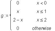
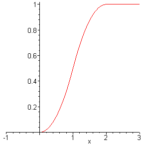
> g:=piecewise(x<0,0,x<=1,x,x<=2,2-x,0);

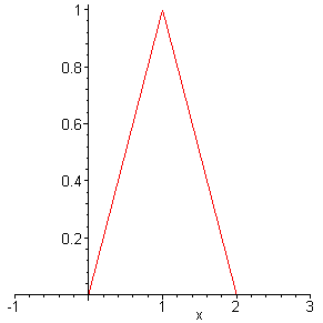
for which Maple allows

> plot(g, x = -1..3);

Moreover, we can implement those analyses so necessary in learning calculus.

> limit(g, x = 1, left);
> limit(g, x = 1, right);
> limit(g, x = 1);

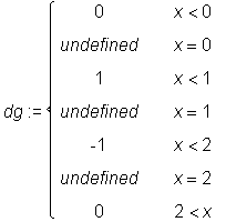
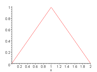
The derivative of g(x) is the piecewise function

> dg := diff(g, x);

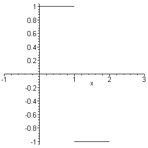
whose graph is obtained by

> plot(dg, x = -1..3, discont = true, color=black);

Furthermore, the indefinite integral of g(x) is obtained as the piecewise defined G, with G given by

> G := int(g, x);

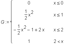
and with graph given by

> plot(G, x = -1..3);

A comparison to Release 3, where most users would have defined g(x) as a Maple procedure, is informative. Using a new name to be consistent with Corollary One of the Large Law (use distinct names for each significant output), we write the procedure

> g3 := proc(x)
> if x<0 then 0
>   elif x<=1 then x
>   elif x<=2 then 2-x
>   else 0
> fi;
> end:

> g3(0.5);

but does not allow plotting. Observe:

> plot(g3(x),x = 0..2);

Error, (in g3) cannot evaluate boolean

> g3(x);

Error, (in g3) cannot evaluate boolean

> plot('g3(x)',x=0..2);

The quotes prevent g3(x) from evaluating before the plot command is called and has a chance to give x a numerical value. Alternatively, plot the function g3 instead of the formula g3(x), that is:

> plot(g3,0..2);

However, we are now into the great overhead of programming procedures, and remembering the different syntax for plotting a function as contrasted to plotting an expression. This extra syntax burden typically obscures the point of the example of the piecewise continuous function.

We conclude with an illustration of another way of defining g3(x) so as to return unevaluated if the argument is not numeric. Like the quotes, this device is useful in other contexts (e.g., defining a function whose output is the result of a call to fsolve, and which is compatible with plot.) It is provided for the sake of the instructor who wishes to have a fuller understanding of the tools being used for instruction.

> gg := proc(x)
>   if type(x,numeric) then
>     if x<0 then 0
>       elif x<=1 then x
>       elif x<=2 then 2-x
>       else 0
>     fi;
>     else 'gg'(x)
>   fi;
> end:

> gg(.3);
> gg(x);

But surely the improved functionality for piecewise in Release 4 is the true ally of the classroom.

Author: Robert J. Lopez
Original file location: http://www.math.utsa.edu/mirrors/maple/mplrjl01.htm